Support Vector Machine Algorithm (SVM) – Understanding Kernel Trick

For a better understanding, the blog has been split into two parts, the former gives conceptual clarity of Support Vector Machine (SVM) & Kernel Trick and the latter gives a mathematical explanation to the same. The blog also entails a complete modelling of the Support Vector Machine Algorithm using Python which will give us more confidence to embrace the algorithm and the concept.

Understanding SVM and SVM Kernel Trick

Before we decipher SVM Kernel Trick, let us first go over few basic concepts:

1. Support Vector Machine (SVM) and Support Vectors

2. Linearity, Non-Linearity, Dimensions and Planes

3. Kernel and Kernel methods

A Support Vector Machine (SVM) is a supervised machine learning algorithm which can be used for both classification and regression problems. Widely it is used for classification problem. SVM constructs a line or a hyperplane in a high or infinite dimensional space which is used for classification, regression or other tasks like outlier detection. SVM makes sure that the data is separated with the widest Margin.

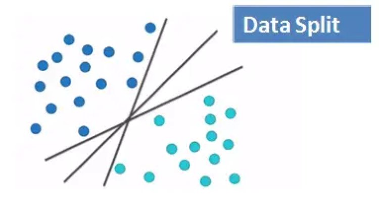
SVMs maximize the margin around the separating hyperplane.

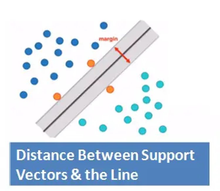
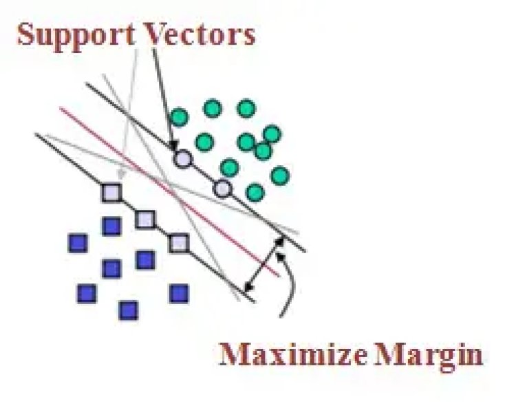
Support Vectors: Support vectors are the data points that lie farthest to the decision surface (or hyperplane). They are the data points which are most difficult to classify. They have a direct impact on the optimum location of the decision surface.

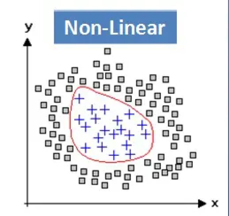
Linearity and Non-Linearity: On a Plane, a linear function is a function where the graph is a straight line. The line can go in any direction, but it’s always a straight line. However, a non-linear function has a shape that is not a straight line.

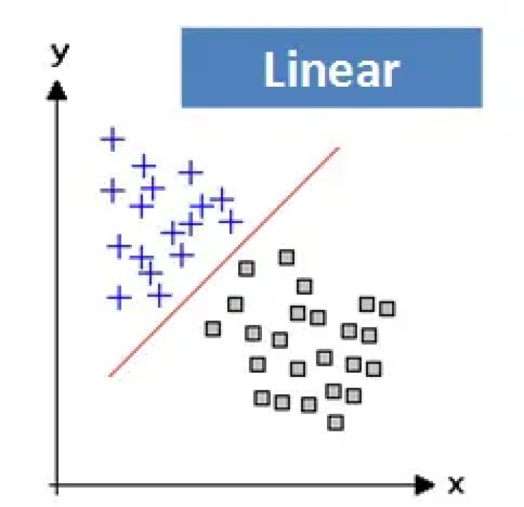
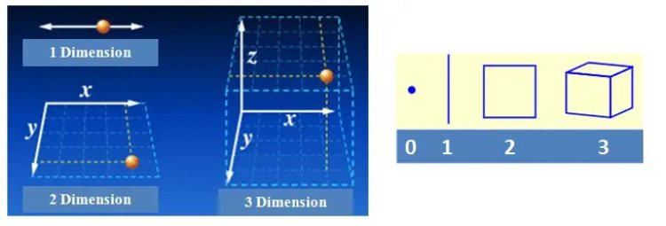
Dimensions: In simple terms, a dimension of something is a particular aspect of it. Examples: width, depth and height are dimensions. A line on a plane is one dimension, considering the edges a square has two dimensions and a cube has three dimensions.

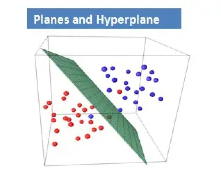
Planes and Hyperplane: In one dimension, a hyperplane is called a point. In two dimensions, it is a line. In three dimensions, it is a plane and in more dimensions we call it a hyperplane.

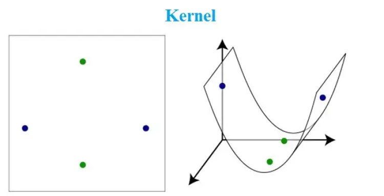
Kernel: A kernel is a method of placing a two dimensional plane into a higher dimensional space, so that it is curved in the higher dimensional space. (In simple terms, a kernel is a function from the low dimensional space into a higher dimensional space.)

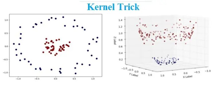
After understanding the above it is now easier to relate and understand the Kernel Trick. We now know that SVM works better with two dimensional space which are linearly separable.

However, for a non-linear data SVM finds it difficult to classify the data. The easy solution here is to use the Kernel Trick. A Kernel Trick is a simple method where a Non Linear data is projected onto a higher dimension space so as to make it easier to classify the data where it could be linearly divided by a plane. This is mathematically achieved by Lagrangian formula using Lagrangian multipliers. (More details in the following mathematical section)

Modelling SVM using Python

The Dataset used for modelling has been taken from UCI machine learning repository. We have opted for Car Evaluation Data Set to model the algorithm.

Quick bite about the dataset: The dataset has 1728 rows and 7 columns (1728, 7). The dataset deals with Car’s acceptability rate which is determined as per below parameters:

Price: Overall price of the car

Buying: Buying price of the car

Maint: Maintenance cost of the car

Doors: Number of doors in the car

Persons: Capacity on the number of persons it can carry

Lug_boot: Luggage boot space available in the car

Safety: Estimated safety in the car

The Outcome generated has been further segregated into 4 classes: unacceptable, acceptable, good and very good which will evaluate and determine the car’s user acceptability rate.

Coding

Voila!! We have got an amazing accuracy score of 99.3 percent with just 3 misclassifications. Our model is highly accurate and robust.

We can see that our model has successfully performed with 6 dimensional space. How is it 6 dimensions? – The 6 parameters or predictors are nothing but dimensions of the algorithm. The data used here is linearly separable, however the same concept is extended and by using Kernel trick the non-linear data is projected onto a higher dimensional space to make it easier to classify the data.

Advantages of Support Vector Machine

• Training of the model is relatively easy
• The model scales relatively well to high dimensional data
• SVM is a useful alternative to neural networks
• Trade-off amongst classifier complexity and error can be controlled explicitly
• It is useful for both Linearly Separable and Non-linearly Separable data
• Assured Optimality: The solution is guaranteed to be the global minimum due to the nature of Convex Optimization

Disadvantages of Support Vector Machine

• Picking right kernel and parameters can be computationally intensive
• In Natural Language Processing (NLP), a structured representation of text yields better performance. However, SVMs cannot accommodate such structures(word embedding)

SVM Applications

There are various applications of Kernel trick few of them are

• Geostatistics: It is a branch of statistics concentrating on spatial or spatiotemporal datasets. It was originally created to predict the probability distributions of ore grading at mining operations. Now it is applied in diverse disciplines including petroleum geology, hydrogeology, hydrology, meteorology, oceanography, geochemistry, geometallurgy, geography, forestry, environmental control, landscape ecology, soil science, and agriculture (specifically in precision farming).
• Inverse distance weighting: Type of deterministic method for multivariate interpolation with a known scattered set of points. The values assigned to unknown points are calculated with a weighted average of the values existing at the known points.
• 3D Reconstruction: Process of capturing the shape and appearance of real objects.
• Bioinformatics: An interdisciplinary field that involves molecular biology, genetics, computer science, mathematics and statistics. Software tools and methods are developed to understand biological data better.
• Chemoinformatics: Application of computational and informational techniques over the field of chemistry to solve a wide range of problems.
• Information Extraction: Acronym as IE, It is a method of automated extraction or retrieval of structured information from an unstructured and semi-structured text documents, databases and websites.
• Handwriting Recognition: Acronym as HWR, It is the ability of a computer system to receive and interpret the handwritten input comprehensibly from different sources such as a letter paper documents, photographs, touch-screens and other devices.

The Kernel Trick Mathematically

Our basic idea of SVM and Kernel trick is to find the plane which can separate, classify or split the data with maximum margin as possible. The margin is also called street width. The distance from a point〖(x〗_0,y_0) to a line: Ax+By+c = 0 is: |Ax_0 + By_0 +c|/sqrt(A2+B2), so, The distance between H0 and H1 is then: |w•x+b|/||w||=1/||w||, so The total distance between H1 and H2 is thus: 2/||w||

In order to maximize the margin, we thus need to minimize ||w||. With the condition that there are no data points between H1 and H2: xi •w+b ≥ +1 when yi =+1 xi •w+b ≤ –1 when yi =–1 Can be combined into: yi (xi •w) ≥ 1

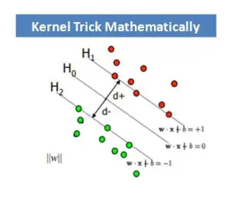
We can intuitively observe that we are trying to optimize the margin or street width by maximizing the distance between support vectors. An optimization problem typically consists of either maximizing or minimizing a real function by systematically choosing input values from within an allowed set and computing the value of the function. Also we are trying to achieve the same with a constraint in mind where the support vectors should be away from the street and not on or in between the street. Hence we can say that this is a typical constrained optimization problem or situation.

This can be solved through Lagrangian formula or lagrangian multipliers. Let us first find the margin or decision boundary for linearly separable plane and then solve with Lagrange multipliers.

• The decision boundary must classify all the points correctly

• The decision boundary can be ascertained by solving the subsequent constrained optimization problem

• As this is a constrained optimization problem. Solving it requires Lagrange multipliers

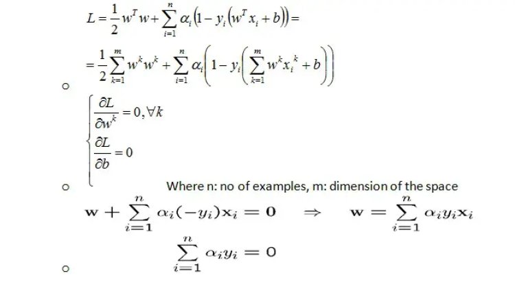
• The Lagrangian is

– ai≥0

– Note that ||w||² = wΤw

• Gradient with respect to w and b

Setting the gradient of L w.r.t. w and b to zero, we have

However for Non-Linearly separable problems

• We allow the “error” xi in classification, it is based on the output of the discriminant function wTx+bo
• xi approximates the number of misclassified samples

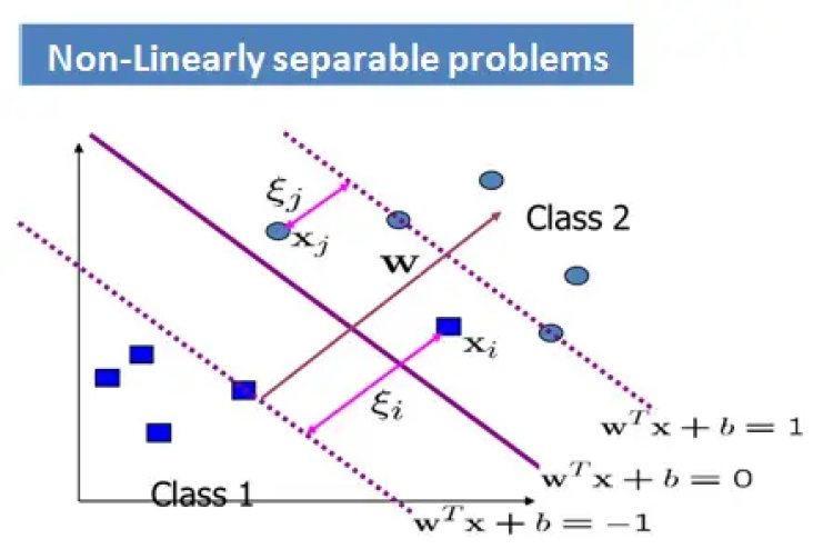
Now the Optimization Problem becomes:

With α and μ Lagrange multipliers, POSITIVE

Extending the same to a Non-Linear margin or decision boundary

We need to transform xi to a higher dimensional space to make our life easier

• Input space: the space where the point xi are located
• Feature space: the space of f(xi) after transformation

Why do we need to transform?

• Linear operation present in the feature space is equivalent to non-linear operation in the input space
• Classification can become easier with a proper transformation.

This can be illustrated with an XOR problem, where adding a new feature of x1x2 makes the problem linearly separable.

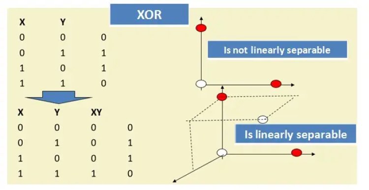
So now as per SVM optimization problem,

The data points appear only as inner product (Xi Xj).

As long as we can compute the inner product in the feature space, we do not require the mapping explicitly. This is called Kernel Trick.

Several common and known geometric operations (angles, distances) can be articulated by inner products. We now can define the kernel function K by

The Kernel Trick can be illustrated with an example:

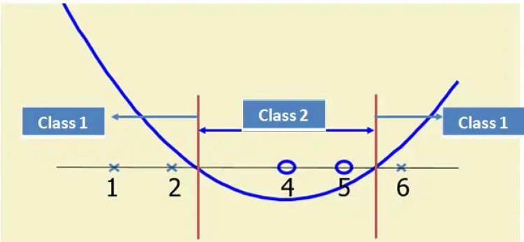
• Suppose we have 5 one Dimensional data points with 1, 2, 6 as class 1 and 4, 5 as class 2

We use the 2nd degree polynomial kernel

• K(x,y) = (xy+1)2
• C is set to 100

• We first find ai (i=1, …, 5)
• By using a Quadratic problem solver, we get

a1=0, a2=2.5, a3=0, a4=7.333, a5=4.833

Note that the constraints are indeed satisfied

The support vectors are {x2=2, x4=5, x5=6}

• The discriminant function is

b is found by solving f(2)=1 or f(5)=-1 or by f(6)=1,

All three would give b=9

Few Popular Kernels: The most tricky and demanding part of using SVM is to choose the right Kernel function because it’s very challenging to visualize the data in n-dimensional space. Few popular kernels are:

• Fisher Kernel: It is a kernel function that analyses and measures the similarity of two objects. This is done on the basis of sets of measurements for each object and a statistical model.
• Graph Kernel: It is a kernel function that computes an inner product on graphs.
• Polynomial Kernel: It is a kernel commonly used with support vector machines (SVMs). It is also used with other kernelised models that symbolizes the similarity of vectors in a feature space over polynomials of the original variables, allowing learning of non-linear models.
• Radial Basis Function Kernel (RBF): It is a real-valued kernel function whose value depends only on the distance from the origin, or distance from some other point called a centre.

Visit DataMites if you are planning to do Data Science course with Machine Learning, Python, Statistics.