What is Simple Linear Regression
Discover what Simple Linear Regression is, how it works, and its applications in data analysis. Learn the basics, formula, and real-world examples of this fundamental statistical method.

Simple Linear Regression (SLR) is one of the most fundamental techniques in statistics and machine learning. It is widely used to model the relationship between two variables: one independent (predictor) and one dependent (outcome). Despite its simplicity, this method is powerful for understanding patterns, making predictions, and serving as a foundation for more advanced algorithms. In this article, we will explore the basics of simple linear regression, its assumptions, how it works, and its applications in real-world scenarios.
Understanding Simple Linear Regression
Simple Linear Regression is a supervised learning algorithm used for predicting numerical outcomes. It examines the relationship between one independent variable (predictor) and one dependent variable (target).
The general mathematical formula is:
Y=β0+β1X+ϵ
Where:
- Y = Dependent variable (the outcome we want to predict)
- X = Independent variable (predictor)
- β₀ = Intercept (value of Y when X = 0)
- β₁ = Slope (the change in Y for one unit change in X)
- ε = Error term (difference between predicted and actual values)
This linear relationship enables data scientists to draw a regression line that best fits the data points while minimizing prediction errors. By 2025, global investments in artificial intelligence are expected to reach $200 billion, with major focus areas including AI model development, infrastructure, and application software.
Key Assumptions of Simple Linear Regression
For Simple Linear Regression (SLR) to produce reliable and accurate predictions, several statistical assumptions need to be satisfied. These assumptions ensure that the model accurately represents the relationship between the independent and dependent variables. Let’s explore each in detail:
1. Linearity
SLR assumes a linear relationship between the independent variable (X) and the dependent variable (Y). This means that any change in X should result in a proportional change in Y. If the relationship is non-linear, the model may underperform, producing biased predictions. Visual tools like scatter plots or residual plots are commonly used to verify linearity.
2. Independence
Each observation in the dataset should be independent of the others. This means that the value of one data point should not influence or be influenced by another. Violation of independence, such as in time-series data with autocorrelation, can distort the model’s coefficients and reduce predictive accuracy. The Durbin-Watson test is often used to check for autocorrelation.
3. Homoscedasticity
Homoscedasticity refers to the assumption that the variance of errors (residuals) remains constant across all levels of the independent variable. If the residuals variance changes (a condition known as heteroscedasticity), it can lead to unreliable estimates of coefficients and invalid statistical tests. Residual plots are commonly used to detect heteroscedasticity.
4. Normality of Residuals
The residuals (differences between observed and predicted values) should be approximately normally distributed. Normality is important for conducting hypothesis tests and creating confidence intervals around predictions. Q-Q plots, histograms, and statistical tests like the Shapiro-Wilk test are used to check residual normality.
Why These Assumptions Matter
Violating any of these assumptions can lead to:
- Biased predictions – The model may systematically over- or under-predict.
- Reduced accuracy – Errors and variability increase, making predictions less reliable.
- Misleading inferences – Hypothesis testing and conclusions drawn from the model may be incorrect.
Ensuring these assumptions are met is essential for developing a reliable, interpretable, and effective Simple Linear Regression model. According to Statista, the artificial intelligence market surpassed several billion U.S. dollars in 2025, marking a significant increase from 2023. This rapid growth is expected to continue, with the market projected to exceed the trillion-dollar mark by 2031.
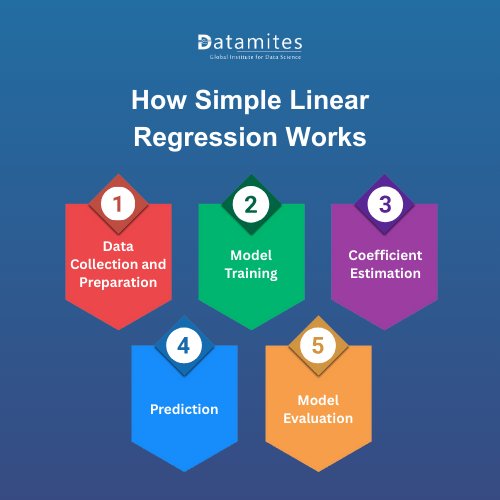
How Simple Linear Regression Works
Simple Linear Regression (SLR) models the relationship between one independent variable (predictor) and one dependent variable (outcome). Despite its simplicity, it follows a structured process to ensure accurate and interpretable predictions. Let’s explore each step in detail:
1. Data Collection and Preparation
The first step in building an SLR model is gathering relevant data. This involves:
- Handling Missing Values: Filling in gaps with techniques like mean, median, or mode imputation.
- Managing Outliers: Identifying and treating extreme values that can skew the regression line.
- Visualizing Data: Using scatter plots to check for linear relationships between the independent and dependent variables.
Proper data preparation is crucial for ensuring the model’s accuracy and reliability.
2. Model Training
Once the data is ready, the model is trained to find the best-fitting line that represents the relationship between the variables.
- Ordinary Least Squares (OLS) is the most commonly used method.
- OLS works by minimizing the sum of squared differences between the predicted values and actual observed values.
This process identifies the line that best captures the underlying pattern in the data.
3. Coefficient Estimation
The next step is to estimate the regression coefficients:
- Intercept (β₀): The predicted value of Y when X is zero.
- Slope (β₁): The change in Y for a one-unit increase in X.
These coefficients not only help make predictions but also provide insight into how strongly the independent variable influences the dependent variable.
4. Prediction
After training, the regression equation can be used to predict new outcomes:
Y = β₀ + β₁X
By substituting new values of X into the equation, you can estimate the corresponding values of Y. For example, predicting a student’s exam score based on the number of study hours.
5. Model Evaluation
To ensure the model performs well, it’s evaluated using metrics such as:
- R² (Coefficient of Determination): Measures how much of the variation in Y is explained by X.
- Mean Squared Error (MSE): Indicates the average squared difference between predicted and actual values.
- Root Mean Squared Error (RMSE): Provides error magnitude in the same units as Y, making it easier to interpret.
Strong performance on these metrics ensures that the model is both accurate and generalizes well to new data.

Applications of Simple Linear Regression
Simple Linear Regression has a wide range of practical applications across industries:
- Business: Forecasting sales revenue based on advertising spend or pricing strategies.
- Healthcare: Predicting patient outcomes using a single factor like age or blood pressure.
- Finance: Estimating stock prices using one economic indicator.
- Education: Analyzing the effect of study hours on student performance.
- Marketing: Understanding customer behavior by analyzing one key metric like website visits versus purchases.
Its straightforward nature and clear interpretability make SLR ideal for tasks where variables are expected to have a linear relationship. According to Precedence Research, the global natural language processing market was valued at USD 30.68 billion in 2024 and is projected to grow from USD 42.47 billion in 2025 to around USD 791.16 billion by 2034, registering a CAGR of 38.4% during the period from 2025 to 2034.
Refer these below articles:
- Python Libraries for Machine Learning
- Artificial Intelligence and Neural Network
- How Gradient Boosting Works in Machine Learning
Enhance Simple Linear Regression Model Performance
While Simple Linear Regression is straightforward, its performance can be enhanced with the following strategies:
- Handling Outliers – Remove or transform extreme values that distort the regression line.
- Feature Scaling – Standardize or normalize input data for better model stability.
- Residual Analysis – Examine residual plots to check assumptions and identify patterns.
- Data Transformation – Apply logarithmic or polynomial transformations if the relationship is slightly nonlinear.
- Cross-Validation – Split data into training and test sets to ensure the model generalizes well on unseen data.
Simple Linear Regression is a cornerstone of machine learning, offering a clear and interpretable method to model the relationship between one independent variable and a dependent variable. Its simplicity makes it an ideal starting point for beginners while still providing value in real-world predictive tasks.
Read these below articles:
Artificial Intelligence is transforming sectors like IT, healthcare, finance, education, transportation, and the startup ecosystem in Hyderabad. By improving efficiency, supporting smarter decision-making, and driving innovation, the city is quickly emerging as a leading AI hub in India. For students and professionals alike, pursuing an Artificial Intelligence course in Hyderabad provides access to promising career opportunities in AI, machine learning, and data science.
DataMites provides a comprehensive Artificial Intelligence course in Pune, tailored to suit both beginners and professionals seeking career growth. The Courses is accredited by reputable organizations such as IABAC and NASSCOM FutureSkills, offering globally recognized, industry-relevant training. Alongside expert-led lessons, DataMites offers extensive career support, including resume building, interview coaching, and placement assistance, enabling learners to confidently pursue successful careers in Machine Learning and Artificial Intelligence.
