Linear Regression Algorithms

Definition:

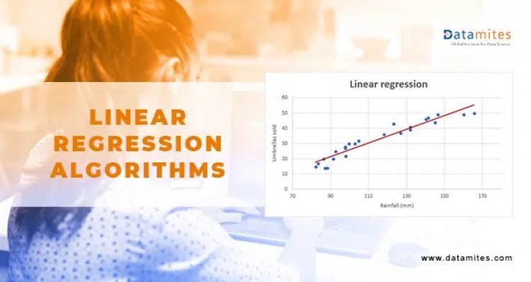
Linear Regression is a supervised machine learning algorithm that describes the linear relationship between predictors and target variables. It is a statistical method for modeling relationships between dependent variables, with a given set of independent variables. It is understood that the two variables are linearly related
It will solve only the regression problem. With the help of a line equation, y = mx + c
which is called the best fit line.
y = mx + c
Where, y = dependent variable (Target variable)
x = independent variable (data points)
m = slope
c = intercept
Let us consider the example of car length and its price, which are directly proportional to each other. If the length of the car is increased the price of the car is also increased.
Assume the red line passing through the origin, to be the best fit line. The equation for the line is given by y = mx + c, where c=0 because it’s passing through the origin. So, the equation becomes Ȳ=mx.

Step to calculate best fit line

• In the above graph, we have data points on the random location of the graph and the best fit line passing through the origin (which can be called prediction or Ȳ).
• First, we calculate the error for the best fit line.
• For that, we will estimate the distance of all points from the line, which is the sum of the distance of all the points from the best fit line.
• And that sum of distance should be minimum.
• Whichever line gives you the minimum error is your best fit line.

To calculate the errors, we have a function called the cost function.

Also called as mean square error or loss function or error.
n = number of data points (observations)
Ȳ = mean point present on best fit line (basically line is Ȳ)
Y = points that are far from the best-fit line (actual data points)

By using this function, we will calculate the error. We have to minimize cost function value. Whichever line will give you minimum value (error) is your best fit line.

Let’s understand this Mathematically:

We have two equations:
y=x (Actual value) Ȳ=mx (predicted value)
We will calculate cost function for two m(slope) value. For m=1, m=0.5
For m=0.5
for m=0.5, x= 1
y = 1
Ȳ = 0.5 * 1 = 0.5
For m=0.5, x=2
y =2
Ȳ = 0.5 * 2 = 1
For m= 0.5, x = 3
y = 0.5 * 3 = 1.5
now for m=0.5, x= 1,2,3, calculate cost function
Cost function = 1 / (2 * 3) * ((1 – 0.5 )2 + (2 – 1 )2 + (3 – 1.5 )2)
= 1/6 * (0.25 + 1 + 2.25)
= 3.5/6
= 0.58
For m=0.5 mean square error is 0.58.

For m=1
For m=1, x=1
y=1
Ȳ = (1) * (1) = 1
For m = 1, x = 2
y=2
Ȳ = (1) * (2) = 2
For m = 1, x = 3
Y = 3
Ȳ = (1) * (3) = 3
Calculation of cost function for m=1, x=1,2,3
Cost function = 1/ (2 * 3) * ((1 – 1)2 + (2-2)2 + (3-3)2 )
= 1/6 * (0)
= 0
For m=1, mean square error is 0.

Just like that, algorithms will calculate the cost function for different m(slope) values and plot a graph between the cost function and the m value.

Gradient descent curve

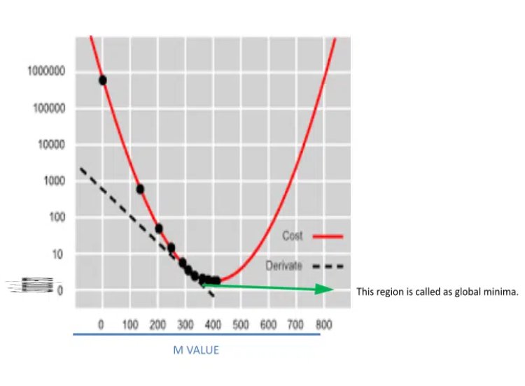
Gradient Descent Curve is a graph between cost function/ error and slope values of data points. In this algorithm, we will put error values for each m value and search for minimum error / global minima where the cost function value is minimum. And using them value which has a minimum error algorithm will create the best fit line. So that the error between the actual and predicted value is minimum.

You can also read: Support Vector Machine Algorithm (SVM) – Understanding Kernel Trick

Now suppose we found (error vs slope) point on the upper region of the graph and for finding global minima we have to move down
For that, we use Convergence Theorem
m=m-(∂m/dm)×∝
Where is the Learning rate
(∂m/dm) is derivative of slope
m is slope
Now to find the derivative of point “A” we have to draw a tangent from point “A”. That depicts the derivative of point “A”

• The next step is to identify if this slope /point “A” is the negative slope or positive
• For that perceive the direction to which the right-hand side of the tangent is pointing towards.
• Suppose it points towards a downward direction then it’s a negative slope
• In case it points towards an upward direction then it’s a positive slope
• Assuming that the left-hand side points toward a down direction which makes it a positive slope
• Now the value of point “A” will be negative because point “A” is tangent to the right-hand side thereby pointing toward a downward direction that is the negative slope. So its derivative is also negative.

For negative value. Equation of Convergence theorem will be

m=m-(-ve)×∝

                      m=m+ve×∝(small)

We must take the value of (Alpha) small as we want our point to move slowly toward global minima rather than the higher value where the point jumps from one part of the graph to other parts (the distance between two points will be high and we don’t want that) and we will not reach the global minima even after many iterations.

Coming to the equation
This equation indicates if your slope (a derivative of slope) is negative then you have to increase your m value then only you will reach the global minima
What if your slope (a derivative of slope) is positive?
The equation will be as follows:

m=m-(+ve)×∝

                  m=m-ve×∝(small)

This equation indicates whether your slope (a derivative of slope) is positive, in which case you have to decrease your m value to reach the global minima.

• That m(slope) value will be used to create a best-fit line for which the error is minimum that is global minima
• That is where you have to stop training the model.
• As the number of features increases from the (slope) value, the dimension will also increase.
• The greater the value for a specific feature the more important the feature will be.

This is all about the internal working of Linear algorithms. How the algorithm decides which line is the best fit line.

DataMites provides global valid data science and artificial intelligence courses along with certification.