Theoretical approach to PCA with python implementation

INTRODUCTION

Data scientists often get data which have huge number of dimensions(independent variable) which leads to 2 major problems.

1) Increase in computational time

Majority of the machine learning algorithms rely on the calculation of distance for model building and as the number of dimensions increases,it becomes more and more computation-intensive to create a model out of it.For example,if we have to calculate the distance between two points in just one dimension,like two points on the number line,we’ll just subtract the coordinate of one point from another and then take the magnitude:

Distance= x1-x2

What if we need to calculate the distance between two points in two dimensions?

The same formula translates to: Distance= √(x1-x2)2+(y1-y2)2
What if we need to calculate the distance between two points in three dimensions?

The same formula translates to: Distance= √(x1-x2)2+(y1-y2)2+(z1-z2)2
And for N-dimensions,the formula becomes: Distance= √ (a1-a2)2+(b1-b2)2+(c1-c2)2+..+(n1-n2)2

This is the effort of calculating the distance between two points.Just imagine the number of calculations involved for all the data points involved.

One more point to consider is that as the number of dimensions increases,points are going far away from each other.This means that any new point that comes when we are testing the model,is going to be farther away from our training points.This leads to a less reliable model,and it makes the model overfitted to the training data.

2) Hard (or almost impossible) to visualise the relationship between features

As stated above,humans can not comprehend things beyond three dimensions.So,if we have an n-dimensional dataset,the only solution left to us is to create either a 2-D or 3-D graph out of it.Let’s say for simplicity,we are creating 2-D graphs.Suppose we have 1000 features in the dataset.That results in a total (1000*999)/2= 499500 combinations possible for creating the 2-D graph.

The above effects are known as the curse of dimensions.

Is it possible for humans to analyse each graph???

The questions that we need to ask at this point are:

• Are all the features really contributing to decision making?
• Is there a way to come to the same conclusion using a lesser number of features?
• Is there a way to combine features to create a new feature and drop the old ones?
• Is there a way to remodel features in a way to make them visually comprehensible?

The answer to all the above questions is – Dimensionality Reduction technique.

What is a Dimensionality Reduction Technique?

Dimensionality reduction is a feature selection technique using which we reduce the number of features to be used for making a model without losing a significant amount of information compared to the original dataset.In other words,a dimensionality reduction technique projects a data of higher dimension to a lower-dimensional subspace.

When to use Dimensionality Reduction? Dimensionality reduction shall be used before feeding the data to a machine-learning algorithm to achieve the following:

• It reduces the size of the space in which the distances are calculated,thereby improving machine learning algorithm performance.
• It reduces the degrees of freedom for our dataset avoiding chances of overfitting.
• Reducing the dimensionality using dimensionality reduction techniques can simplify the dataset facilitating a better description,visualisation.

Principal Component Analysis:

The principal component analysis is an unsupervised machine learning algorithm used for feature selection using dimensionality reduction techniques.As the name suggests,it finds out the principal components from the data.PCA transforms and fits the data from a higher-dimensional space to a new,lower-dimensional subspace This results into an entirely new coordinate system of the points where the first axis corresponds to the first principal component that explains the most variance in the data.PCA is used for feature extraction.

What are the principal components?

Principal components are the derived features which explain the maximum variance in the data.The first principal component explains the most variance,the 2nd a bit less and so on.Each of the new dimensions found using PCA is a linear combination of the old features.

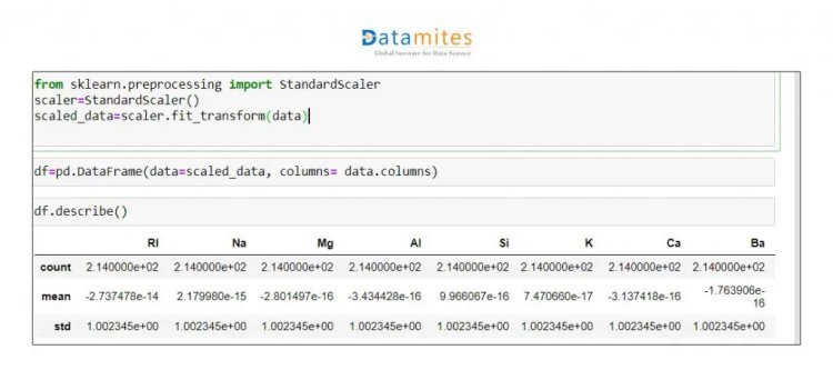
PCA assumes that the mean of all the individual columns is zero and the standard deviation is 1.So,before applying PCA,the data should be pre-processed appropriately.

How Principal component analysis works?

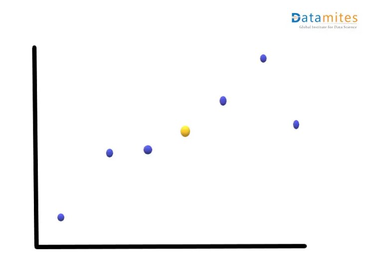
Step1:- Consider a 2-dimensional dataset Let’s plot this on the XY plane and calculate the average of the magnitude of all the points.Blue ones are the actual points and the yellow one is the average point.

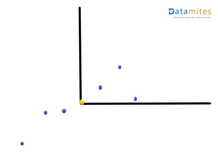
Step 2:- Move the points so that the average point is on the origin.This is called a parallel translation.Although the coordinates of the points have changed,the corresponding distances among them remain the same.

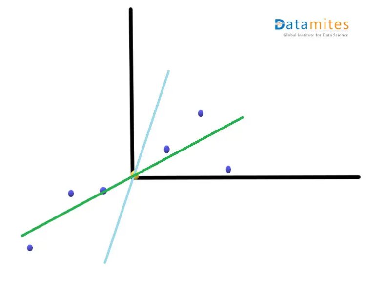
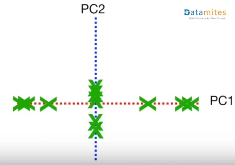
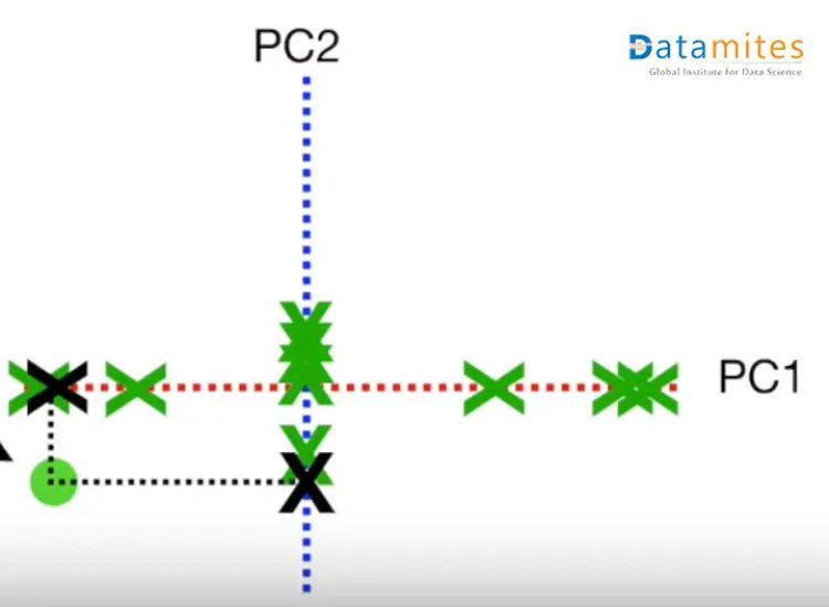
Step 3:- Create the best fit line for the new data points.We first start with a random line(the blue one) and then try to find the best fit line(the green one) so that the distance from individual data points is minimum and consequently the distance from the origin is maximum.This best fit line is called Principal component1 or PC1.PC2 is a line perpendicular to the PC1.Then the axes PC1 and PC2 are rotated in a way that PC1 becomes the horizontal axis

Then based on the sample points the new points are projected using PC1 and PC2.Thus we get the derived features.

What is the optimum number of Principal components needed?

This is done by the explained variance ratio.It represents the amount of variance each principal component is able to explain.

For example,suppose if the square of distances of all the points from the origin that lies on PC1 is 50 and for the points on PC2 it’s 5.

EVR of PC1= DistanceofPC1points(DistanceofPC1points+DistanceofPC2points)
= 5055
= 0.91

EVR of PC2= DistanceofPC2points(DistanceofPC1points+DistanceofPC2points)
= 555
= 0.09

Thus PC1 explains 91% of the variance of data.Whereas,PC2 only explains 9% of the variance.Hence we can use the only PC1 as the input for our model as it explains the majority of the variance.
In a real-life scenario,this problem is solved using the Scree Plots.

Scree Plots:

Scree plots are the graphs that convey how much variance is explained by corresponding Principal components.

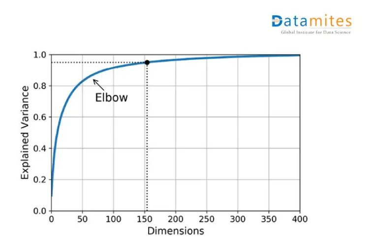
As shown in the given diagram,around 75 principal components explain approximately 90 % of the variance.Hence,75 can be a good choice based on the scenario

Python Implementation

Step 1 Initial Package import

import pandas as pd
import numpy as np
import matplotlib.pyplot as plt
%matplotlib inline

Step 2 we are using the free glass dataset.

#The objective is to tell the type of glass based on the amount of other elements present.
data = pd.read_csv(‘glass.data’)

Step 3 Getting the first 5 rows of data

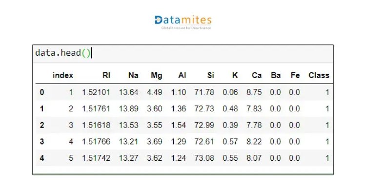
Step 4 Check for missing data

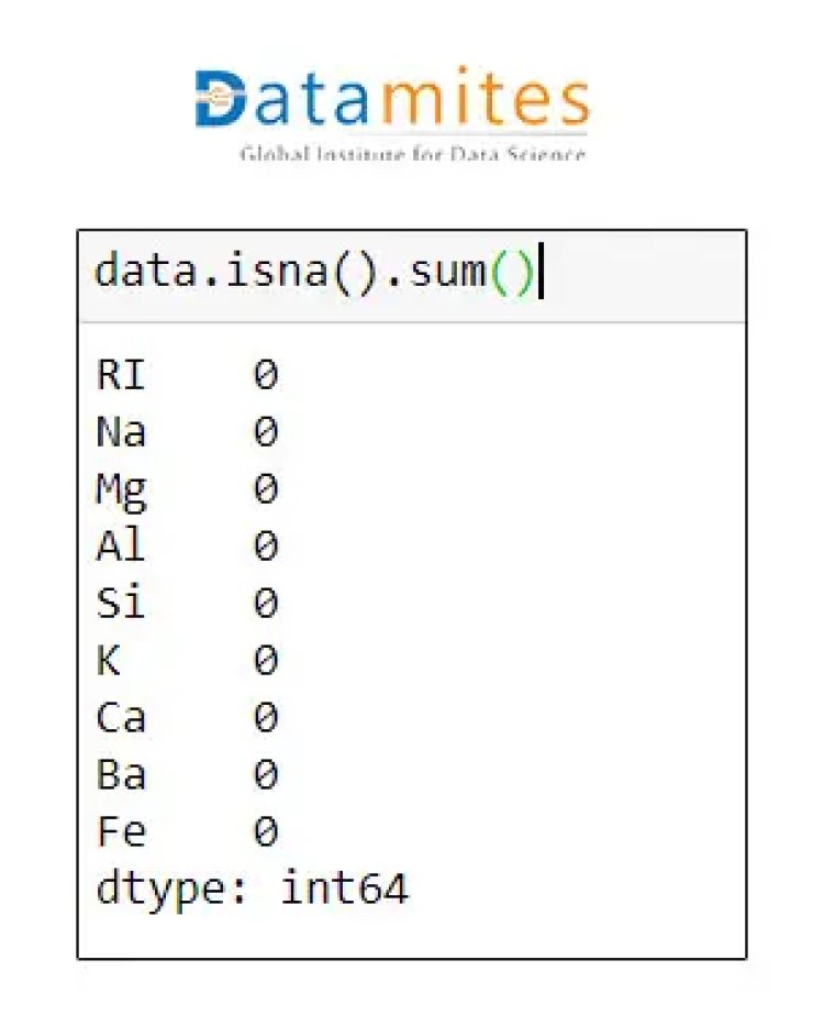
Step 5 We will standardise this data as all the data is on a different scale.

Step 6 Apply PCA to whole dataset and check Explained Variance Ratio

from sklearn.decomposition import PCA
pca = PCA()
principalComponents = pca.fit_transform(df)
plt.figure()
plt.plot(np.cumsum(pca.explained_variance_ratio_))
plt.xlabel(‘Number of Components’)
plt.ylabel(‘Variance (%)’) #for each component
plt.title(‘Explained Variance’)
plt.show()

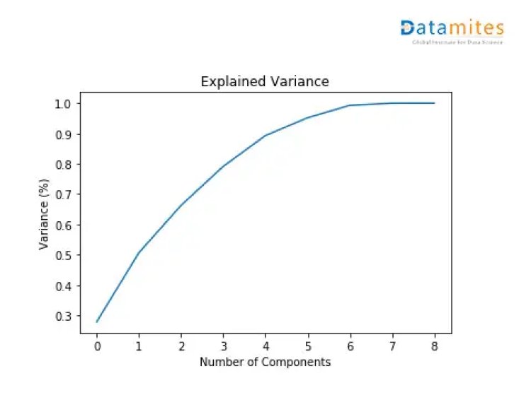
From the diagram above,it can be seen that 4 principal components explain almost 90% of the variance in data and 5 principal components explain around 95% of the variance in data.

So,instead of giving all the columns as input,we’d only feed these 4 principal components of the data to the machine learning algorithm and we’d obtain a similar result.

Step 7 Apply PCA with n_components=4

pca = PCA(n_components=4)
new_data = pca.fit_transform(df)

#This will be the new data fed to the algorithm.

principal_Df = pd.DataFrame(data = new_data
,columns = [‘principal component 1’,‘principal component 2',’principal component 3',’principal component 4’])
principal_Df .head()

Step 8 Model Building

After selecting PCA components ,create model out of it.To test the model performance on unseen data,save the model as .pickle file and do the predictions
Import pickle
ilename = ‘finalized_model.sav’
pickle.dump(model,open(filename,‘wb’))

#some time later…

#load the model from disk

loaded_model = pickle.load(open(filename,‘rb’))
result = loaded_model.score(X_test,Y_test)
print(result)

Here,we see that earlier we had 9 columns in the data earlier.Now with the help of Scree plot and PCA,we have reduced the number of features to be used for model building to 4.This is the advantage of PCA.It drastically reduces the number of features,thereby considerably reducing the training time for the model.

Pros of PCA:

Correlated features are removed.
Model training time is reduced.
Overfitting is reduced.
Helps in better visualizations
Ability to handle noise

Cons of PCA

The resultant principal components are less interpretable than the original data
Can lead to information loss if the explained variance threshold is not considered appropriately.