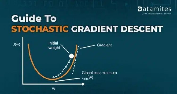
A Complete Guide to Stochastic Gradient Descent (SGD)

In the space of loss function, we have to reach a point that gives us the minimum loss. The Approach could be varying but we need to choose one, which gives us the optimum value for the problem we are working on. Scientists found one of the profound approaches called Stochastic Gradient Descent. Before diving further into it, let’s understand some basic concepts of mathematics which work under the hood.

Differentiation: 

• Single variable differentiation
• Let’s say I have a function f(x) = x^2 + 2x + 3
• differentiation of f(x) : d f(x) / dx = 2x + 2
• if I put x = 2 here, I get a value:
• d f(x) / dx = 6
• The value of 6 signifies that y changed 6 units when x was changed for 1.
• So dy/dx or d f(x)/ dx is intuitive, is how much y changes as x changes for a particular given point.

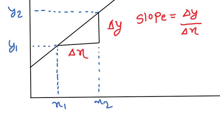
From the above diagram (y2 – y1) / (x2 – x1) = Δ(y)/Δ(x)

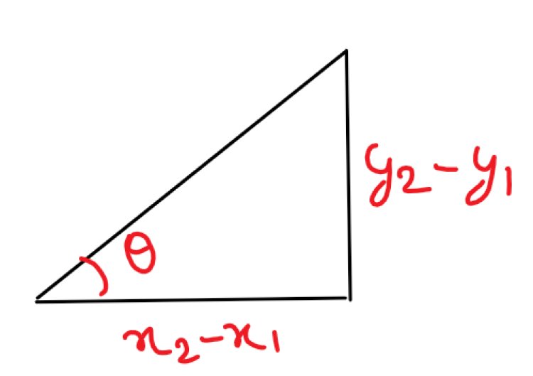
And, from trigonometry, we know Tanθ = perpendicular/base

Hence, Tanθ = (y2 – y1)/(x2 – x1)

        Tanθ = Δy / Δx 

So, Tanθ at any point of the graph signifies the value changed by y is when x is changed with an infinitely small value. i.e. limit x -> 0.

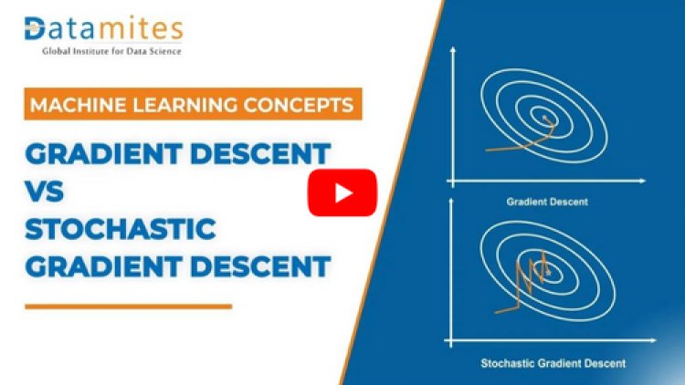
Gradient Descent & Stochastic Gradient Descent Explained

Maxima and Minima:

The purpose of any optimizer is to smoothly get us to the minimum point of the loss value in the loss surface

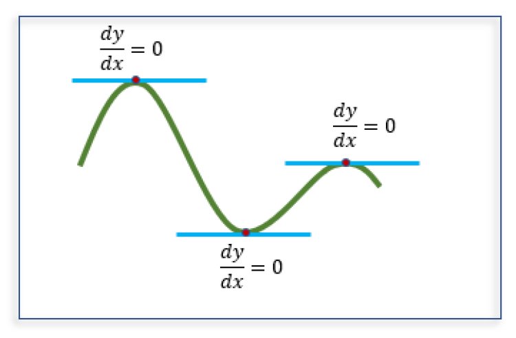
Both at the maxima and minima point, as θ = 0, hence Tan(θ) = 0

It can be also interpreted in this way that when at the maxima or minima point, there is absolutely no change of y with a change in x.

Let us take an example and understand:

If f(x) = x² – 3x + 2 and if we need to find x for which the value of the equation is either maximum or minimum, then :

df(x)/dx = 0

df(x)/dx = 2x – 3 = 0

x = 1.5

so, 1.5 is the value for which the equation will be either maxima or minima.

Let’s find out what exactly it is,

f(1.5) = 2.25 – 4.5 + 2 = -0.25

let’s take a value less than 1.5, say 1

f(1) = 1 – 3 + 2

f(1) = 0

so f(1.5) < f(1)

hence it means that x = 1.5 is the minima for f(x) = x² – 3x + 2.

So, finding the optimum point looks quite easy, isn’t it? but the problem comes when we encounter some compound equation like f(x) = log(1 + exp(ax)), 

then df/dx = (a*exp(ax)/(1 + exp(ax)) = 0 and from here things starts to look quite complex.

Refer this article: Support Vector Machine Algorithm (SVM) – Understanding Kernel Trick

Then how to get the value for which my equation becomes minimum? The one hot solution is Gradient Descent and Stochastic Gradient Descent.

Gradient Descent: It is an algorithm that starts from a random point on the loss function and iterates down the slope to reach the global minima of the function. The weight of the algorithm is updated once every data point is iterated for the calculation of the loss that occurred.

W_{new =} W_old – eta(dL/dX)

After every iteration, the value of the slope is calculated i.e. dL/dx. and the new weight is calculated using the formula W_{new =} W_old – eta(dL/dX)

eta🡪 Learning Rate

W_old 🡪 Previous old weight

W_new🡪 Updated the new weight

dL/dX 🡪 The gradient value that we got after the iteration.

So, Iteration after iteration, a new weight is calculated and it goes on till the value of W_new and W_old becomes equal meaning we have reached a point where the gradient/slope has become zero.

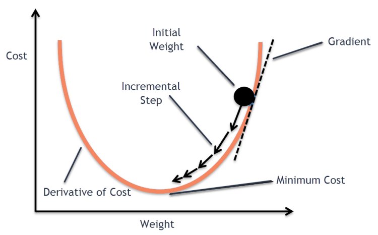
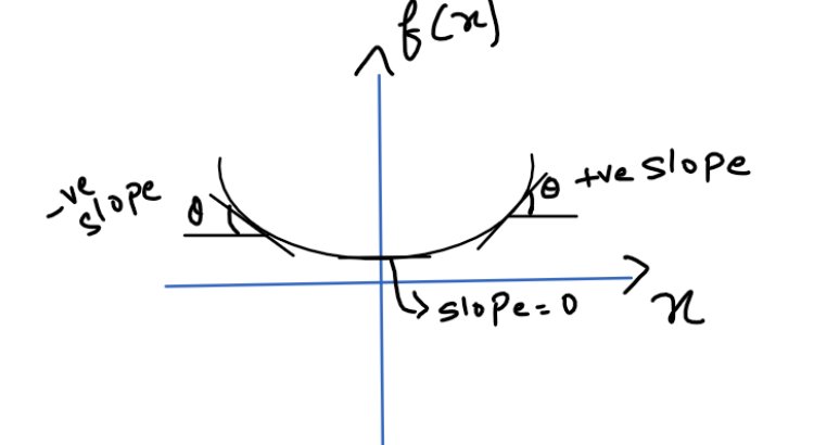
As you move closer and closer to the minima, the value of the slope starts to reduce and eventually becomes 0 which means we have reached to minima point and the slope changes its sign from +ve to -ve as we cross the minima.

Read this article: A Complete Guide to Linear Regression Algorithm in Python

Learning rate(eta):

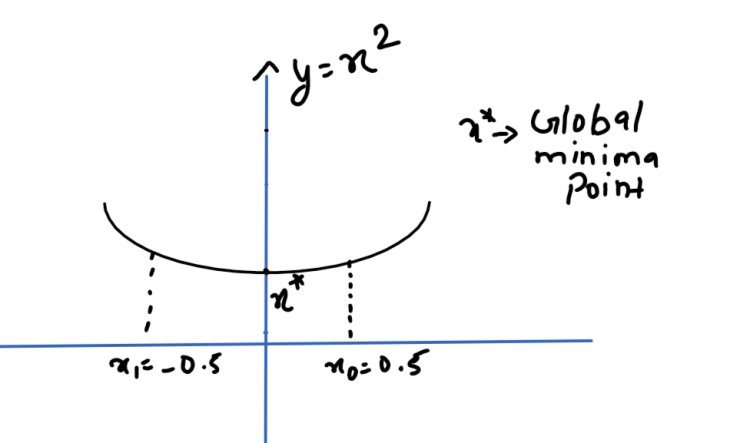
Lets take x₀ = 0.5 and learning rate (eta) = 1

X₁ = X₀ – eta[df/dx]

X₁ = 0.5 –(2 * 0.5)

X₁ = 0.5 – 1

X₁ = – 0.5

So X₁ jumped the global minima point x* and came to the left side of the graph. So to prevent these unwanted hops, we apply a learning rate usually of the order 0.001 or 0.01 so that the steps taken are small and we don’t surpass the global minima point.

Also Refer this article: The Complete Guide to Recurrent Neural Network

Stochastic Gradient Descent :

The major drawback of the Gradient Descent Algorithm is to calculate the squared residuals of all the data points available. Let’s say we have 20000 data points with 10 features. Then the gradient will be calculated concerning all the features for all the data points in the set. So the total number of calculations will be 20000 * 10 = 200000. For attaining global minima, it is common for an algorithm to have 1000 iterations. So now, the total number of computations performed by the system will be 200000 * 1000 = 200000000. This is a very large computation that consumes a lot of time and hence Gradient descent is slow over the huge dataset.

To get rid of this problem, Instead of considering all the data points, we only choose one point with random probability, and then dL/dx is calculated and further Xnew is calculated. Hence the computational complexity goes down and global minima can be reached easily over the large dataset.

Mini batch SGD is also one of the techniques in which we take chunks of data from the dataset and df/dx is computed based on that.

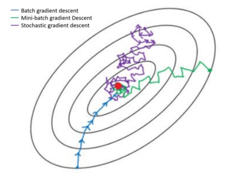
The GD is a much smoother approach to reach the global minima, followed by mini-batch GD and finally Stochastic Gradient Descent

Being a prominent data science institute, DataMites provides specialized training in topics including ,artificial intelligence, deep learning, Python course, the internet of things. Our machine learning at DataMites have been authorized by the International Association for Business Analytics Certification (IABAC), a body with a strong reputation and high appreciation in the analytics field.

Whats is ADAM Optimiser?

What is Neural Network & Types of Neural Network