What is a Gradient Descent?

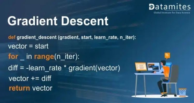
In machine learning, the optimization of algorithms is very important to train ML models and neural networks. The accuracy increases with each iteration and the cost function with gradient descent acts as an optimizing function. The model will continue to adjust all the parameters till the function is close to or equal to 0. 

A cost function is a function that traverses all the data points in a dataset and then goes through the POC (Point of Convergence) where the value of the cost function is minimum.

For a linear function y = mx+c, the slope of the line adjudged as m c is the intercept on the y-axis. The cost function is the line of best fit, which is required to calculate the error between the actual output and the predicted output using the MSE (Mean Squared Error) formula. The gradient descent algorithm is very much similar to a polynomial function which is convex in nature.

Taking dy/dx of a particular section of the curved cost function we can determine the slope of the function at that particular point. Taking the example of a convex up function, the slope will be higher in magnitude i.e., the curve will be a sleeper and it should gradually decrease when we reach the POC (Point of Convergence) where the slope, m will be 0.

To better understand Gradient Descent, we need to learn about Learning Rates. This is also known as alpha and in simpler terms, step size. It is defined as the number of steps that are taken to reach the minimum value. Usually, it is a small number, and it is updated on the basis of the change in the cost function. Higher learning rates usually have the disadvantage of going past the POC (Point of Convergence) i.e., the minimum value. Hence, smaller learning rates are generally preferred to reach the POC, the minimum value. The only disadvantage to this is a higher number of iterations and more time required by smaller learning rates.

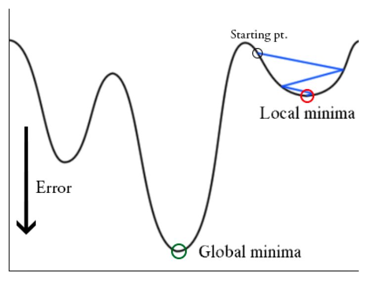
The Cost function establishes the discrepancy between the actual y and predicted y. The Loss function is another name for this. Providing feedback improves the machine learning model’s efficacy by enabling it to adjust the parameters, reduce error, and find the local or global minimum. It iterates regularly until the cost function is close to or equal to zero, moving in the direction of the steepest descent (or the negative gradient). Hence, the name Gradient Descent. Although often used interchangeably, the terms Cost function and Loss function are somewhat different. The cost function with the help of MSE determines the average error. Whereas, the loss function determines the error of one particular sample.

There are 3 different types of Gradient Descent. 

• Batch Gradient Descent
• Stochastic Gradient Descent
• Mini-batch Gradient Descent.

Refer to the article to know: Support Vector Machine Algorithm (SVM) – Understanding Kernel Trick

Batch Gradient Descent

Also referred to as a training epoch, batch gradient descent calculates the error for each data point and adds it up. It then updates the model in the end after all the data points have been evaluated.

This has a high efficiency pertaining to time complexity for small and average-sized datasets but as the size of the dataset increases, the processing time increases. It generates a balanced convergence and stable error gradient. But in lieu of finding the convergence point, batch gradient descent often mistakes the local minima to be the global minima.

Read this article: Exploratory Data Analysis

Stochastic Gradient Descent

This algorithm runs the epochs for each data point within a dataset and it changes the training parameters one at a time.

Stochastic Gradient Descent has a very efficient space complexity as it occupies less memory due to the training of single data points. It results in higher speeds and effective storage, but it increases the loss when it comes to the efficiency of the algorithm. Changing parameters repeatedly often results in noisy gradients. The added advantage to this is that it helps in evading the local minima and finding the global minima.

Refer to the article: Introduction to Boxplots

Mini-Batch Gradient Descent

Mini-batch gradient descent is a combination of Batch Gradient Descent and Stochastic Gradient Descent. Here the algorithm divides the dataset into several smaller batches and updates training parameters for each of the batches. This is a highly effective way to find the Point of Convergence as it restores the computational efficiency of the Batch Gradient Descent without losing out on the efficient space complexity provided by the Stochastic Gradient Descent.

This concludes the blog on gradient descent. You would have gotten a general idea of what the gradient descent is and what are its types. 

Being a prominent data science institute, DataMites provides specialized training in topics including Data Analytics course, machine learning, deep learning, Python course, the internet of things. Our artificial intelligence at DataMites have been authorized by the International Association for Business Analytics Certification (IABAC), a body with a strong reputation and high appreciation in the analytics field.

Gradient Descent & Stochastic Gradient Descent Explained

Whats is ADAM Optimiser?

What is Neural Network & Types of Neural Network