What is Multiple Linear Regression in Machine Learning?

Machine learning is built upon mathematical and statistical techniques that help systems learn patterns from data. One of the most widely used methods in predictive modeling is Multiple Linear Regression (MLR). Unlike simple linear regression, which analyzes the relationship between a single independent variable and a dependent variable, multiple linear regression evaluates how two or more independent variables influence an outcome.

In this article, we will explore what multiple linear regression is, how it works, its assumptions, applications in machine learning, and the techniques to improve model performance.

Understanding the Basics of Multiple Linear Regression

Multiple Linear Regression is a supervised learning algorithm primarily used for regression tasks. Its goal is to model the linear relationship between a dependent variable (target) and multiple independent variables (features).

The general mathematical representation is:

                       Y=β0​+β1​X1​+β2​X2​+...+βn​Xn​+ϵ

Where:

• Y = Dependent variable (outcome)
• X₁, X₂, …, Xₙ = Independent variables (predictors)
• β₀ = Intercept
• β₁, β₂, …, βₙ = Coefficients that represent the weight of each predictor
• ε = Error term (residuals)

This model assumes a linear relationship between the variables, which can be represented by fitting a line (or a hyperplane in higher dimensions) that minimizes prediction errors. By 2030, Artificial Intelligence is expected to increase global GDP by 26%, adding approximately $15.7 trillion to the world economy.

Assumptions of Multiple Linear Regression

For Multiple Linear Regression models to deliver accurate and trustworthy results, certain statistical assumptions need to be satisfied. These assumptions ensure that the model captures relationships correctly and avoids misleading interpretations. Let’s look at them in detail:

1. Linearity

The relationship between the dependent variable (outcome) and independent variables (predictors) should be linear. This means changes in predictors should result in proportional changes in the response variable. If the relationship is non-linear, the model may underperform or fail to detect patterns. Data visualization techniques like scatter plots and residual plots can help check this assumption.

2. Independence

Each observation in the dataset should be independent of the others. In simple terms, the outcome of one observation should not influence another. Violating this assumption, such as in time-series or panel data, can lead to autocorrelation, which distorts the regression results. Techniques like the Durbin-Watson test are commonly used to detect autocorrelation.

3. Homoscedasticity

Homoscedasticity refers to the assumption that the variance of residuals (errors) is constant across all levels of the independent variables. If the variance of errors increases or decreases with predictors (heteroscedasticity), the model may give biased standard errors, leading to unreliable confidence intervals and hypothesis tests. Visualizing residuals versus fitted values can help check this condition.

4. Normality of Errors

The residuals (differences between predicted and actual values) should follow a normal distribution. This assumption is particularly important for hypothesis testing and confidence interval estimation. Normality can be assessed using Q-Q plots, histograms, or statistical tests like the Shapiro-Wilk test.

5. No Multicollinearity

Independent variables should not be highly correlated with each other. Multicollinearity makes it difficult to determine the unique contribution of each predictor to the outcome. It also inflates the variance of coefficients, leading to unstable estimates. Variance Inflation Factor (VIF) is a popular method to detect multicollinearity, and techniques like feature selection or regularization can help reduce it.

Why These Assumptions Matter

Violating one or more of these assumptions can result in:

• Biased coefficients – making the model unreliable.
• Reduced predictive accuracy – lowering the model’s effectiveness in real-world applications.
• Invalid inferences – leading to incorrect business or research decisions.

By meeting these assumptions, practitioners can develop robust, interpretable, and reliable regression models. According to Markets and Markets, the generative AI market is set for explosive growth, expected to rise from USD 71.36 billion in 2025 to USD 890.59 billion by 2032, registering a remarkable CAGR of 43.4% during the forecast period.

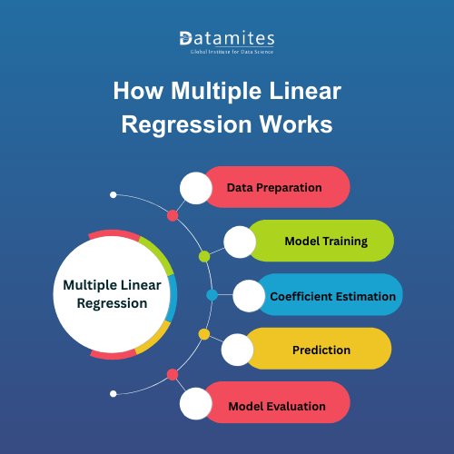
How Multiple Linear Regression Works

Multiple Linear Regression (MLR) works by modeling the relationship between one dependent variable and multiple independent variables. The process involves a series of structured steps that ensure the model is both accurate and reliable. Let’s break it down in detail:

1. Data Preparation

The first step in Multiple Linear Regression is preparing the dataset. This includes:

• Handling Missing Values: Filling missing entries with mean, median, or mode, or using advanced imputation techniques.
• Scaling Features: Standardizing or normalizing numerical features ensures variables with large ranges don’t dominate the model.
• Encoding Categorical Variables: Converting categorical data (e.g., “Male/Female” or “Yes/No”) into numerical values using one-hot encoding or label encoding.

Proper preprocessing ensures the data is clean and ready for regression analysis.

2. Model Training

Once the data is ready, the regression model is trained. The most common method is Ordinary Least Squares (OLS), which finds the best-fitting line (or hyperplane in higher dimensions) by minimizing the sum of squared residuals — the differences between actual and predicted values.

This step essentially teaches the model how the predictors influence the outcome.

3. Coefficient Estimation

In this stage, the model calculates the regression coefficients (β values) for each independent variable.

• A positive coefficient means the predictor has a direct relationship with the dependent variable.
• A negative coefficient means the predictor has an inverse relationship.

These coefficients help interpret the strength and direction of the relationships between variables.

4. Prediction

After training, the model can be used to make predictions on new data points. By plugging in the values of independent variables into the regression equation:

Y = β₀ + β₁X₁ + β₂X₂ + … + βₙXₙ + ε

The model predicts the dependent variable. For example, given house size, location, and number of rooms, the model can predict the price of a house.

5. Model Evaluation

To measure how well the model performs, evaluation metrics are used, such as:

• R² (Coefficient of Determination): Explains the proportion of variance in the dependent variable captured by the model.
• Mean Squared Error (MSE): Measures the average squared difference between predicted and actual values.
• Root Mean Squared Error (RMSE): Provides error in the same units as the dependent variable, making it easier to interpret.

Strong performance in these metrics indicates that the model generalizes well to unseen data.

Applications of Multiple Linear Regression in Machine Learning

Multiple Linear Regression has a broad range of real-world applications:

• Predictive Analytics: Estimating sales revenue based on marketing spend, pricing, and seasonal factors.
• Healthcare: Predicting patient health outcomes using age, medical history, and lifestyle variables.
• Finance: Modeling stock prices, interest rates, or credit scores using multiple economic indicators.
• Education: Analyzing student performance based on study hours, attendance, and socioeconomic factors.
• Business Decision-Making: Understanding the impact of multiple variables like pricing, promotions, and customer demographics on sales performance.

Its high interpretability makes Multiple Linear Regression particularly useful in industries that demand explainable AI. According to Grand View Research, the global wearable AI market was valued at USD 26,879.9 million in 2023 and is expected to reach USD 166,468.3 million by 2030, expanding at a CAGR of 29.8% between 2024 and 2030.

Refer these below articles:

• What is Information Retrieval (IR) in Machine Learning?
• Data Preprocessing in Machine Learning
• Tools for Visualizing Machine Learning Models

Techniques to Improve Multiple Linear Regression Models

Although Multiple Linear Regression is a powerful technique, its accuracy and reliability can be improved using the following strategies:

• Feature Selection – Remove irrelevant or redundant predictors using techniques like Recursive Feature Elimination (RFE) or LASSO regression.
• Addressing Multicollinearity – Use Variance Inflation Factor (VIF) to detect correlated predictors and drop or combine them.
• Transforming Variables – Apply log, square root, or polynomial transformations to capture nonlinear patterns.
• Regularization – Techniques like Ridge and LASSO regression add penalty terms to reduce overfitting.
• Cross-Validation – Split data into training and validation sets to ensure generalization on unseen data.
• Scaling Features – Standardize or normalize data for better coefficient interpretation.

Multiple Linear Regression is a foundational algorithm in machine learning that enables data-driven predictions using multiple variables. By understanding its assumptions, working principles, and real-world applications, practitioners can build accurate and interpretable models. With improvements like feature selection and regularization, Multiple Linear Regression continues to remain relevant in solving business and research problems.

Read these below articles:

• Top IT Courses in Jalandhar
• Top IT Courses in Vellore
• Top IT Courses in Thanjavur

Bangalore (Bengaluru) has quickly established itself as a leading hub for artificial intelligence in India and across Asia. The city benefits from a strong mix of renowned educational institutions, a large pool of skilled professionals, a vibrant startup ecosystem, active investor participation, and government initiatives that encourage innovation. In such an environment, enrolling in an Artificial Intelligence course in Bangalore can be highly advantageous. With the growing need for AI experts, competitive salary opportunities, and diverse learning options, the right program can significantly accelerate your career advancement.

Datamites Artificial Intelligence course in Hyderabad delivers a well-structured training program designed for both beginners and professionals. The curriculum focuses on hands-on learning with real-time projects, guidance from industry experts, and dedicated placement assistance, making it ideal for those looking to advance in Hyderabad’s growing technology ecosystem. On completion, learners receive globally recognized certifications from IABAC and NASSCOM FutureSkills, boosting their career prospects and helping them stand out in the competitive AI job market.