A Complete Guide to Decision Tree Algorithm in Python

Decision Tree is one of the powerful algorithms that come under the non-parametric Supervised Learning Technique. A Decision Tree can be used for Regression and Classification tasks alike. It is a tree-based algorithm that divides the entire dataset into a tree-like structure based on certain conditions. This intuitive method is easy to understand and highly efficient in solving any kind of classification and regression problem.

Let’s discuss the decision tree in detail in this blog.

Before seeing how a decision tree works, we will understand what is decision tree and why we need a decision tree.

What is a decision tree?

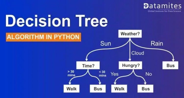
It is a tool that creates a tree-like structure of a given dataset with branches to represent the decision-making steps that result in a probable outcome. It presents the algorithm with conditional control statements. The structure of the decision tree includes root nodes, internal nodes, and leaf nodes. The root node represents the entire dataset where it takes a feature to split the dataset into branches consisting of internal nodes for a further split.

Decision Tree Algorithm:

It is a non-parametric supervised ML Algorithm which can be used for both classification and regression tasks. It is the most versatile algorithm that works on simple nested if-else conditions. While constructing the Decision tree, it uses an algorithm called ID3 which always selects the right feature to split the dataset into a decision tree. It is very powerful and works great with complex datasets. And it is easy to interpret.

Read this article to know: Support Vector Machine Algorithm (SVM) – Understanding Kernel Trick

How does it work?

This algorithm works by dividing the whole dataset into a tree-like structure based on some rules or conditions and then gives predictions based on those conditions. It uses the tree representation to solve the problem in which each leaf node corresponds to class labels and attributes (features) are represented on the internal node of the tree for the further split. The tree is the pattern that the model identifies after getting trained with the given data. So, using that pattern predicts the output.

The decision algorithm tree splits the dataset by taking a feature in the root node. There could be many features in the dataset. So, choosing the feature for splitting becomes important, as the right feature can reach the leaf node quickly. The leaf node helps in taking the decision. So how does it select the right feature to make the split? It uses metrics such as Entropy, Information Gain or Gini Index to do that.

Refer this article to know: A Complete Guide to Logistic Regression Algorithm in Python

Terminologies in Decision Trees:

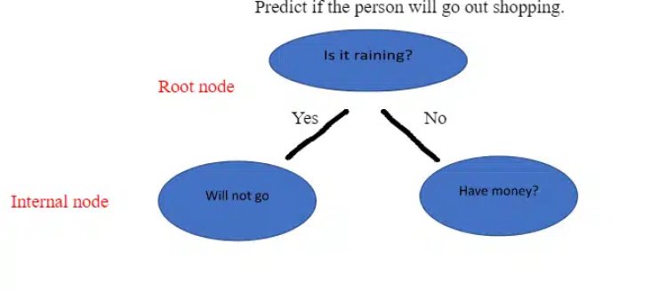
Root Node: It is the starting node that represents the population and further gets divided into two or more sets.
Internal Node / Decision Node: These are the sub nodes that will be again split.
Terminal Node/Leaf Node: These are the final node that cannot be split further.
Pruning: It is the process of cutting (removing) down the unwanted branches (part of the entire tree) from the decision tree.
Branch: Each branch represents an outcome of the test.

There are multiple ways to create a pure split. Based on the type of the target variable, the metrics are differentiated.

• In terms of the categorical target variable, Gini Index or (Entropy) Information Gain is used to measure the quality of the split.
• In terms of the continuous target variable, Variance Reduction can be used.
• Let us look into the metrics used to measure the purity of the split.

Entropy: Entropy is the measure of the purity of the split or we can say it as a measure of uncertainty. The value for entropy can vary from 0 to 1. The entropy is 0 for the node when it has only a single class label for the samples and entropy is 1 when it has an equal number of class labels for the samples. Our aim in creating an ML model is to reduce uncertainty. Hence for any split, if the entropy is closer to zero or zero, we consider that as the best split and the feature which was taken for splitting is the right feature. Entropy is calculated by;

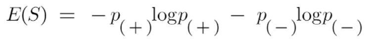
Where
p+ is the probability of a positive class
p– is the probability of negative class
S is the subset of the training set

For eg;

Let’s calculate Entropy for the node with 3yes and 2 no,

E(S) = -3/5 log2(3/5) – 2/5 log(2/5) = 0.78bits

Also refer this article: A Comprehensive Guide to K-Nearest Neighbor (KNN) Algorithm in Python

Information Gain:

Here for a single node, we have calculated Entropy. When we want the entropy for the full dataset, we go for Information Gain which measures the reduction of uncertainty. It also helps in deciding the feature for the root node and decision node.
Information Gain can be calculated by;

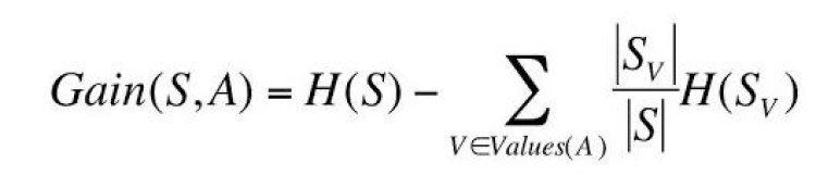
Where
V – possible values of an attribute
S – Set of training data
Sv – Subset of training data

Let’s calculate Information Gain for the below split;

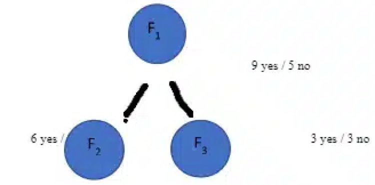
Gain (S, F1)
= [-(9/14) log2(9/14) – (5/14) log2(5/14)] – [ 8/14 – [(6/8) log2(6/8)] + 6/14 – [(3/6) log2(3/6)]]
= 0.94 – 8/14(0.81) – 6/14(1) = 0.049

Measure purity of a node in Decision Tree Algorithm

Gini Index:

Similarly, Gini Index can be used to select the best feature for the split. The value ranges from 0 to 0.5 for Gini Index where if Gini is 0 for any node, then it is the best split having a single class label in the leaf node and if Gini is 0.5, then we have an equal number of class labels which consider as the worst split. Based on these metrics, the decision tree algorithm selects the best feature to have the best split.

Gini Index is calculated by;

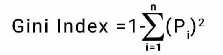
Which is = 1 – [ (P+)2 + (P-)2 ]
Where
P+ – Probability of positive class
P- – Probability of negative class

For eg;

Let’s calculate Gini Index for the node with 3yes and 2 no,

Gini = 1 – [ (3/5)2 + (2/5)2 ] = 0.48

What is One Hot Encoding

Variance Reduction:

This metric calculates the variance for each child node for each split and calculates the variance of each split as the weighted average variance of the child nodes. And choose the split that has the lowest variance.
To calculate the variance;

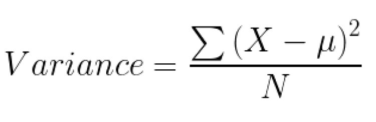
Any split that gives less variance is considered to be the best split.

The important hyperparameters in the Decision Tree:

• Max_depth: This parameter defines how maximum the tree can grow. If the depth is too high then the model would overfit the training data and will cause more testing errors.
• Min_samples_split: It specifies the minimum number of samples for splitting the decision node.
• Min_samples_leaf: It specifies the minimum number of samples to be present in leaf nodes.
• Max_features: This specifies the number of features to be taken for doing the best split.
• Criterion: It measures the quality of the split using ‘Gini’ or ‘Entropy’.

These are the important hyperparameters of the decision tree. So, to improve the performance of the model, we can tune these hyperparameters using GridSearchCV or RandomizedSearchCV to find the optimal values for these hyperparameters.

What is Ensemble Technique?

Implementation of Decision Tree algorithm in Python:

Business Case:
With the given features we need to classify the samples as ‘body’ of ceramics or ‘glaze’ of ceramics.
1. Import the necessary packages:
import pandas as pd
import numpy as np
import matplotlib.pyplot as plt
import seaborn as sns
import warnings
warnings.filterwarnings(‘ignore’)
from scipy import stats

2. Load the dataset
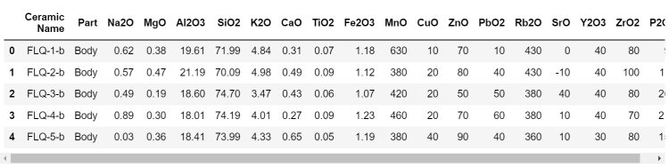
df = pd.read_csv(“Chemical Composion of Ceramic.csv”)
df.head()

3. Do all the basic checks.
df.info()
df.describe()

4. Feature analysis
Target Variable:
Part: a binary categorical variable (‘Body’ or ‘Glaze’)
[A ceramic glaze is an impenetrable covering or coating made of a vitreous material that has been fired into fusion with a ceramic body.]

• Ceramic. Name: name of ceramic types from Longquan and Jingdezhen
• Na2O: percentage of Sodium oxide (wt%)
• MgO: percentage of Magnesium oxide (wt%)
• Al2O3: percentage of Aluminium oxide (wt%)
• SiO2: percentage of Silicon dioxide (wt%)
• K2O: percentage of Potassium oxide (wt%)
• CaO: percentage of Calcium oxide (wt%)
• TiO2: percentage of Titanium dioxide (wt%)
• Fe2O3: percentage of Ferric oxide (wt%)
• MnO: percentage of Manganese(II) oxide (ppm)
• CuO: percentage of Copper(II) oxide (ppm)
• ZnO: percentage of Zinc oxide (ppm)
• PbO2: percentage of Lead(IV) oxide (ppm)
• Rb2O: percentage of Rubidium oxide (ppm)
• SrO: percentage of Strontium oxide (ppm)
• Y2O3: percentage of Yttrium oxide (ppm)
• ZrO2: percentage of Zirconium dioxide (ppm)
• P2O5: percentage of Phosphorus pentoxide (ppm)

These are the features that help in predicting the class labels.

5. Perform EDA for the given data.

6. Let’s perform the feature engineering:

i) Handling the missing values.
We dont have any missing values in this dataset.
ii) Handling the categorical features.
We have one categorical feature ‘Part’ in our dataset. Let’s convert it into a numerical feature.

Let’s apply the Label encoding technique here.

from sklearn.preprocessing import LabelEncoder
le = LabelEncoder()
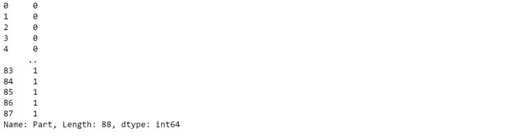
df.Part = le.fit_transform(df[‘Part’])
df.Part

ii) Checking for outliers and handling them.
There are 4 features that have outliers. Let’s handle them.

Handling outliers for Na2O:

IQR = stats.iqr(df.Na2O, interpolation = ‘midpoint’) Inter quantile range #calculating

Q1=df.Na2O.quantile(0.25) of data  #defining 25%

Q3=df.Na2O.quantile(0.75) of data ##defining 75%

min_limit=Q1 – 1.5*IQR minimum limit #setting

max_limit=Q3 + 1.5*IQR maximum limit #setting

replace the outlier with the median of Na2O

df.loc[df[‘Na2O’]>max_limit,’Na2O’]=np.median(df.Na2O)

# MgO

IQR = stats.iqr(df.MgO, interpolation = ‘midpoint’)
Q1=df.MgO.quantile(0.25)
Q3=df.MgO.quantile(0.75)
min_limit=Q1 – 1.5IQR max_limit=Q3 + 1.5IQR
df.loc[df[‘MgO’]>max_limit,’MgO’]=np.median(df.MgO)

# TiO2

IQR = stats.iqr(df.TiO2, interpolation = ‘midpoint’)
Q1=df.TiO2.quantile(0.25)
Q3=df.TiO2.quantile(0.75)
min_limit=Q1 – 1.5IQR max_limit=Q3 + 1.5IQR
df.loc[df[‘TiO2′]>max_limit,’TiO2’]=np.median(df.TiO2)

# MnO

IQR = stats.iqr(df.MnO, interpolation = ‘midpoint’)
Q1=df.MnO.quantile(0.25)
Q3=df.MnO.quantile(0.75)
min_limit=Q1 – 1.5IQR max_limit=Q3 + 1.5IQR
df.loc[df[‘MnO’]>max_limit,’MnO’]=np.median(df.MnO)

We have handled the outliers.

7. Feature Selection:

removing the unwanted feature

df.drop(‘Ceramic Name’, axis=1, inplace=True)

Feature selection based on the correlation between features.

fig, ax = plt.subplots(figsize=(15,15))
sns.heatmap(df.drop(‘Part’,axis=1).corr(),annot=True) # checking for correlation

Removing the highly correlated feature

df.drop(‘CaO’, axis=1, inplace=True)

define X and y

X = df.drop(‘Part’, axis=1)
y = df.Part

splitting data into training and testing set

from sklearn.model_selection import train_test_split
X_train, X_test, y_train, y_test = train_test_split(X,y, test_size=0.25, random_state=42)

Feature Scaling

from sklearn.preprocessing import StandardScaler
scalar = StandardScaler() ## object creation
X_train = scalar.fit_transform(X_train) # scaling independent variables
X_test = scalar.transform(X_test)

check if the data is balanced

df.Part.value_counts()

Creating a DT model with the default parameters from sklearn.tree import DecisionTreeClassifier
DT = DecisionTreeClassifier()
DT.fit(X_train, y_train)

Model prediction

y_pred = DT.predict(X_test)

Model Evaluation

from sklearn.metrics import accuracy_score, f1_score

For testing data

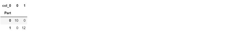
accuracy = accuracy_score(y_test, y_pred)
accuracy
1.0

calculating the f1 score

f1_score(y_test, y_pred)
1.0

confusion matrix

pd.crosstab(y_test, y_pred)

Prediction for training data

tra = DT.predict(X_train)

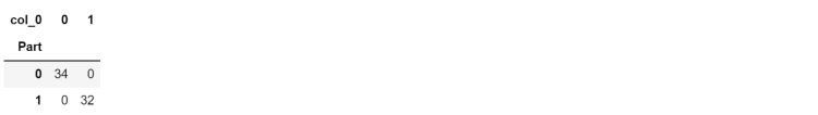
confusion matrix for training data

pd.crosstab(y_train, tra)

Hyper parameter tuning to find the optimal values for parameters for improving the model performance from sklearn.model_selection import GridSearchCV

params = {
“criterion”:(“gini”, “entropy”), #quality of split
“splitter”:(“best”, “random”), # searches the features for a split
“max_depth”:(list(range(1, 20))), #depth of tree range from 1 to 19
“min_samples_split”:(list(range(1, 20))), #the minimum number of samples required to split internal node
“min_samples_leaf”:list(range(1, 20)),#minimum number of samples required to be at a leaf node,we are passing list which is range from 1 to 19
}

initialize a model

tree_clf = DecisionTreeClassifier(random_state=3)#object creation for decision tree with random state 3

Hyper parameter tuning using GridSearchCV

tree_cv = GridSearchCV(tree_clf, params, scoring=”f1″, n_jobs=-1, verbose=1, cv=3)

tree_cv.fit(X_train,y_train) #training data on gridsearch cv
best_params = tree_cv.best_params_ #it will give you best parameters
print(f”Best paramters: {best_params})”) #printing the best parameters

Creating a DT model with the best hyperparameter values

dt_clf = DecisionTreeClassifier(criterion=’gini’, max_depth=1, min_samples_leaf=1,
min_samples_split=2, splitter=’random’)

Model Evaluation

dt_clf.fit(X_train, y_train) # training the model
y_p_test = dt_clf.predict(X_test)
acc_test=accuracy_score(y_test,y_p_test)
acc_test

0.9090909090909091

confusion matrix

pd.crosstab(y_test, y_p_test)

Demystifying Feature Engineering

Advantages:

• It is very intuitive and its simple representation makes it easy to understand.
• This algorithm does not require scaling of data and not much data pre-processing is required.
• It can handle both

Disadvantages:

• Training time is more and it is expensive as the complexity increases.
• It generally leads to overfitting.
• Any change in the data may change the structure of the decision tree.

Conclusion:

The decision Tree Algorithm is used for making numerous business decisions based on past data. These decisions are helpful in predictive modelling to predict the outcomes. Decision trees are used in several fields like data mining, marketing, diagnosis of disease, fraud detection etc. The ease of use and the simplicity is the predominant characteristics of this algorithm.

Being a prominent data science institute, DataMites provides specialised training in topics including machine learning, deep learning, artificial intelligence, the internet of things. Our python Courses at DataMites have been authorised by the International Association for Business Analytics Certification (IABAC), a body with a strong reputation and high appreciation in the analytics field.

Confusion Matrix Machine Learning Foundation