A Guide to Principal Component Analysis (PCA) for Machine Learning
Discover how Principal Component Analysis (PCA) reduces dimensionality, enhances visualization, and improves machine learning models. Learn its key concepts, implementation, and practical applications.
 Thushara C.P

Sometimes there are situations where the dataset contains many features or as we call it High Dimensionality. High dimensionality datasets can cause a lot of issues, the most common issue that occurs is Overfitting, which means the model is not able to generalize beyond the training data. Therefore, we have to employ a special technique called Dimensionality Reduction Technique to deal with this High Dimensionality. One of the best techniques that we use is known as Principal Component Analysis(PCA).
Principal Component Analysis:
Principal Component Analysis is one of the best Dimensionality Reduction Techniques available in Machine Learning. It is a type of feature extraction technique where it retains the more important features and discards the less important ones. The way it works is that it transforms the existing dataset by reducing the number of features and retaining only important features which are called Principal Components while also making sure that it retains as much information as possible from the original Dataset.
The main aim of PCA is to reduce the number of features or variables in a dataset and also retain as much information as possible from the actual dataset.
Steps Involved in PCA:
Step 1: Standardization
In this step, we standardize the range of the values in all the variables to a similar range so that all of them have equal contributions to the analysis.
The main reason why we perform standardization before actually performing the PCA is that PCA is very sensitive to the variance of the original variables in the dataset. The reason is that, if there are features with big differences in their initial range of values then the features with a higher range of values will dominate the overall analysis and PCA will be more biased towards those features. So performing standardization initially can prevent this from happening.
Standardization is done by using the following formula:
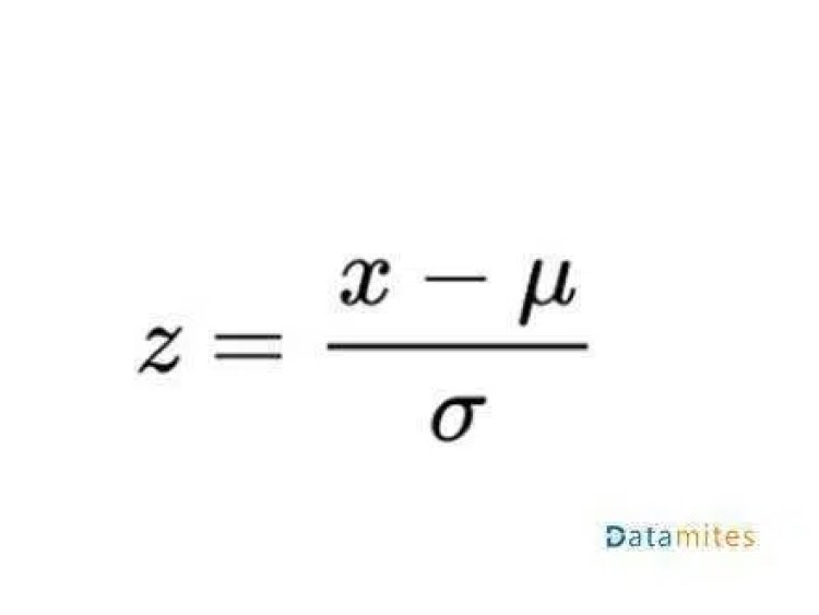
Where x is the Value
- u is the mean of the feature/variable
- α is the Standard Deviation
Once the Standardization is done, and all features are scaled down to a similar range, we will now proceed with the PCA method.
Step 2: Calculate Covariance Matrix
The main aim of this step is to understand the variance of the input data from the mean or in simple terms we try to find if there is any relationship between the features. The reason we do this is that sometimes there are features that are highly correlated and contain similar information. So to find the correlation we compute the Covariance Matrix.
Step 3: Computing the EigenValues and EigenVectors
EigenValues and EigenVectors are part of Linear Algebra and we have to compute them using the Covariance Matrix to generate the Principal Components. Before we proceed, let’s understand the term Principal Component.
Check out the below videos:
What is Sparse Matrix – Machine Learning & Data Science Terminologies
Confusion Matrix Machine Learning Foundation

What is the Principal Component?
In simple terms, Principal Components are the new transformed features or we say the output of the PCA Algorithm is Principal Components.
Usually, the number of PCs is equal to less than the original number of features present in the dataset.
Below are some of the properties of Principal Components:
- PCs should be a linear combination of the variables of the original dataset.
- The PCs are Orthogonal i.e there is zero correlation between a pair of features.
- The Importance of each PC keeps decreasing from PC1 to nth PC meaning, PC1 has the most importance and nth PC has the least importance.
So the PCs are constructed by combining the initial features of the dataset. The process is done in such a way that none of the PCs is correlated with each other and most of the information is squeezed into the first few PCs. For example, let’s say there is a dataset with 10 features and we apply PCA to it. So we get 10 PCs, but the PCA algorithm puts maximum information into the 1st PC and then remains to the 2nd PC and so on. We sort the PCs in the descending order of their EigenVectors to get something like this:
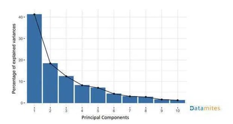
In this way, we organize information into the form of Principal Components thus allowing us to reduce the number of features without losing too much data. So we discard the features that have less variance and consider the new variables which have high variance.
Watch the video: What is PCA ?
What is Vector?

How does PCA create Principal Components?
Principal Components are created in such a way that the 1st PC has the highest possible variance in the dataset. The next PC is constructed similarly but under the condition that it should not be Correlated with the 1st PC and must account for the next largest variance.
This process continues until we get a total of p number of PCs and it should be equal to the number of variables in the original dataset.
Now we know what Principal Components are so let’s get back to EigenValues and EigenVectors. They usually appear in pairs i.e every EigenVector has an EigenValue. EigenValues and EigenVectors are the main reasons behind the creation of Principal Components.
- EigenVectors are nothing but the direction of the axis with maximum Variance which is nothing but the PCs.
- EigenValues are nothing but coefficients attached to the EigenVectors representing the variance in each Principal Component.
So we rank these EigenVectors in the order of their respective EigenValues in descending order. The result is that you get Principal Components in the order of their level of variance.
Step 4: Selecting the Appropriate number of Principal Components
Now that we have the Principal Components the next step is to select the best Principal Components that we require. So basically we select the top PCs based on their respective EigenVectors using the EigenValues. We form a matrix of these vectors called Feature Vector.
Feature Vector is nothing but a matrix with the columns containing the EigenVectors of the newly formed PCs. You could say this is our initial step toward Dimensionality Reduction. So if we decide to keep p EigenVectors(PCs) out of n original number of features of the dataset, then the overall final dataset will only have p number of features.
Step 5: Reload Data along the Principal Component Axes
This is the final step where we just use the newly formed feature vector with the selected EigenVectors(PCs) and then just reorient the data of the original axes to the ones represented by the PCs. This is done by multiplying the Transpose of the feature vectors by the Transpose of the Original dataset.
These are the steps involved in the Whole Principal Component Analysis.
Application of PCA:
- PCA is mainly used as a Dimensionality Reduction Technique for some of the A. I related Applications such as Computer Vision, Image Compression, Facial Recognition, etc.
- It is also used to find any hidden pattern when data has a lot of features.
Advantages and Disadvantages of PCA:
There are plenty of benefits of PCA but it also has some drawbacks.
Advantages:
- It’s very easy to implement and also easy for the computer to compute as well.
- Machine learning Algorithms perform much better when we train the model with the Principal Components instead of Original features from the dataset.
- In Regression-based problems, due to the presence of high dimensional data, the model will tend to overfit. So we use PCA and reduce the feature and therefore prevent the overfitting.
Disadvantages:
- It can be very difficult to interpret and can be difficult to select the most appropriate features after applying PCA.
- Although PCA is very useful in Dimensionality Reduction it comes at the cost of Information loss. So we have to make a compromise between the reduced features and information loss.
Being a leading data science provider, DataMites offers specialised training in subjects like artificial intelligence, machine learning, deep learning, the internet of things, and Python. Our Machine Learning Certification Courses at DataMites is International Association for Business Analytics Certification (IABAC) accredited and holds high value.
The DataMites Machine Learning course provides expert-level training in AI-driven data analysis, enabling computers to learn from experience and execute tasks without explicit programming. Accredited by IABAC and NASSCOM FutureSkills, DataMites is a trusted leader in AI and Machine Learning education, empowering over 100,000 learners globally with a decade of excellence.
For further reference:
BUILD A TENSORFLOW OCR IN 15 MINUTES WITH DEEP LEARNING TECHNOLOGY
A Guide to MLOps (Machine Learning Operations)
Machine Learning Vs Deep Learning